Life Distributions - Page 1 of 4

Life Distributions

Reliability engineers are in many ways like soothsayers - they are expected to predict many things for the semiconductor company: how many failures from this and that lot will occur within x number of years, how much of this and that lot will survive after x number of years, what will happen if a device is operated under these conditions, etc.

To many people, such questions seem overwhelmingly difficult to answer, half-expecting reliability engineers to demonstrate some supernatural powers of their own to come up with the right figures.

Fortunately for reliability engineers, they don't need any paranormal abilities to give intelligent responses to questions involving failures that have not yet happened. All they need is a good understanding of statistics and reliability mathematics to be up to the task.

Reliability assessment, or the process of determining to a certain degree of confidence the probability of a lot being able to survive for a specified period of time under specified conditions, applies various statistical analysis techniques to analyze reliability data. If properly done, a reliability prediction using such techniques will match the survival behavior of a lot, many years after the prediction was made.

A good understanding of life distributions is a must-have for every reliability engineer who expects to exercise sound reliability engineering judgment whenever the need for it arises. A life distribution is simply a collection of time-to-failure data, or life data, graphically presented as a plot of the number of failures versus time. It is just like any statistical distribution, except that the data involved are life data.

By looking at the time-to-failure data or life distribution of a set of samples taken from a given population of devices after they have undergone reliability testing, the reliability engineer is able to assess how the rest of the population will fail in time when they are operated in the field. Based on this reliability assessment, the company can make the decision as to whether it would be safe to release the lot to its customers or not, and what risks are involved in doing so.

All new engineers in the semiconductor industry are acquainted with the bath tub curve, which represents the over-all failure rate curve generally observed in a very large population of semiconductor devices from the time they are released to the time they all fail. The bath-tub curve has three components: the early life phase, the steady-state phase, and the wear-out phase.

The failure rate is highest at the beginning of the early life phase and the end of the wear-out phase. On the other hand, it is lowest and constant in the long steady-state phase at the middle part of the curve. Collectively, these phases make the curve look like a bath tub (where it obviously got its name).

The bath tub curve takes into account all possible failure mechanisms that the population will encounter. Some failure mechanisms are more pronounced in the early life phase (such as early life dielectric breakdown), while others are more pronounced in the steady-state or wear-out phases. Failures that occur in the early life phase are known as infant mortality, which are screened out in production by burn-in.

In real life, it is not always practical to evaluate the failure or survival rate of a population of devices in terms of the bath tub curve. Reliability assessments are often conducted to evaluate only the known weaknesses of a given lot or, if the lot has no known weaknesses, to determine if it is vulnerable to any of the critical failure mechanisms dreaded in the semiconductor industry today.

Such reliability assessments are conducted by running a set of industry-standard reliability tests, generating life data along the way. These life data are then analyzed according to what type of life distribution they fit.

There are currently four (4) life distributions being used in semiconductor reliability engineering today, namely, the normal distribution, the exponential distribution, the lognormal distribution, and the Weibull distribution. Different failure mechanisms will result in time-to-failure data that fit different life distributions, so it is up to the reliability engineer to select which life distribution would best model the failure mechanism of interest.

Life distributions are described mathematically by life distribution functions. Three of these functions are very important descriptors of life distributions, and should be understood by every reliability engineer. These are the cumulative failure distribution function F(t), the failure probability density function f(t), and the curve of failure rate l(t).

The cumulative failure distribution function F(t), or simply cumulative distribution function, gives the probability of a failure occurring before or at any time, t. This function is also known as the unreliability function. If a population of devices is operated from its initial use up to a certain time t, then the ratio of failures, c(t), to the total number of devices tested, n, is F(t). Thus, F(t) = c(t)/n. F(t) is therefore always less than 1, which is consistent with the fact that it's just a probability number after all.

The unreliability function F(t) has an equivalent opposite function - the reliability function R(t). R(t) = 1 - F(t), so it simply gives the ratio of units that are still good to the total number of devices after these devices have operated from initial use up to a time t.

The failure probability density function f(t), or simply probability density function, gives the relative frequency of failures at any given time, t. It is related to F(t) and R(t) by this equation: f(t) = dF(t)/dt = -dR(t)/dt.

The curve of failure rate l(t), also known as the failure rate function or the hazard function, gives the instantaneous failure rate at any given time t. It is related to f(t) and R(t) by this equation: l(t) = f(t)/R(t). Thus, l(t) = f(t)/[1-F(t)].

More details on how these functions describe the various life distributions may be found at Life Distribution Functions.

The Normal Life Distribution

A normal life distribution is one that consists of time-to-failure or life data that constitute a normal distribution. Thus, it is a symmetric bell-shaped curve whose mean, median, and mode are equal. The spread of the normal life distribution is determined by the standard deviation s of its life data. The failure rate of a normal life distribution monotonically increases with time, which is failure rate pattern typically exhibited by failures due to wear-out.

Normal distributions are often a result of the additive effects of random variables. Thus, normal life distributions are generally applicable to failures that are affected by additive factors, such as mechanical system failures that occur as a result of the accumulation of small and random mechanical damage. Such mechanical failures are often observed as the system wears out with use.

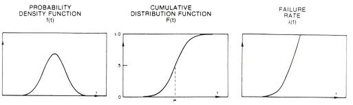
Figure 1. The f(t), F(t), and l(t) of a normal life distribution; source: D. S. Peck and O. D. Trapp, Accelerated Testing Handbook, Technology Associates.

We all know that the over-all failure rate of semiconductors do not increase monotonically with time. In fact, there aren't too many semiconductor failure mechanisms that fit the normal life distribution. Thus, the normal life distribution is generally not used by reliability engineers to model semiconductor survival in the field.

Note, however, that the bath tub curve representing the failure rate curve of semiconductor devices does include a wear-out phase in the end. This wear-out phase, although just the end portion of a semiconductor's life, may be modeled by a normal life distribution.

The Exponential Life Distribution

An exponential life distribution is one wherein the failure rate is constant in time. The exponential life distribution is best applied to the analysis of failures in the steady-state phase of the bath tub curve, during which the failure rate is constant. Other than this, reliability engineers don't use the exponential life distributions a lot, because there are not too many frequently-encountered critical failure mechanisms that exhibit this life distribution.

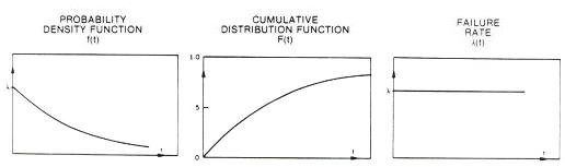
Figure 2. The f(t), F(t), and l(t) of an exponential life distribution; source: D. S. Peck and O. D. Trapp, Accelerated Testing Handbook, Technology Associates.

The Lognormal Life Distribution

The lognormal life distribution is one wherein the natural logarithms of the lifetime data, ln(t), form a normal distribution. Consequently, the life data of a lognormal distribution will also form a straight line if plotted on a lognormal plot, i.e., a plot whose x- and y-axes stand for the cumulative % of failures and the logarithmic scale of time, respectively. The failure rate curve l(t) of a lognormal life distribution starts at zero, rises to a peak, then asymptotically approaches zero again for all values of s.

The lognormal distribution is formed by the multiplicative effects of random variables. Multiplicative interactions of variables are found in many natural processes, and are in fact observed in many frequently-encountered semiconductor failure mechanisms. This characteristic of the lognormal distribution makes it a good choice for the analysis of the failure rates of many semiconductor failure mechanisms.

A notable characteristic of the lognormal distribution is the fact that its median time to failure, t_50%, or the time at which 50% of the samples fail, is equal to e^µ, where µ is the mean of the life data. Thus, t_50%= e^µ.

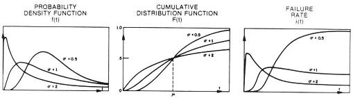
Figure 3. The f(t), F(t), and l(t) of a lognormal life distribution; source: D. S. Peck and O. D. Trapp, Accelerated Testing Handbook, Technology Associates.

The Weibull Life Distribution

The Weibull life distribution was developed by W. Weibull of Sweden to investigate metal fatigue failures. It is described by a location parameter a and a shape factor b, and is similar to the lognormal distribution in many ways. Two of the major differences between them are: 1) the Weibull distribution's probability density function does not start from zero; and 2) its failure rate curve l(t) is monotonically increasing for b > 1 and monotonically decreasing for b < 1.

The Weibull distribution can take on many shapes, depending on the value of the shape factor b. In fact, by varying the value of b, all the phases of the bath tub curve can be modeled by the Weibull distribution. The early life phase, wherein the failure rate decreases with time, can be represented by the Weibull distribution with b < 1. The steady-state phase, wherein the failure rate is constant, can be represented by the Weibull distribution with b = 1. Finally, letting b be > 1 will make the Weibull distribution a model for the wear-out phase, wherein the failure rate increases with time.

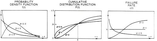
Figure 4. The f(t), F(t), and l(t) of a Weibull life distribution; source: D. S. Peck and O. D. Trapp, Accelerated Testing Handbook, Technology Associates.

The Weibull distribution has become popular in reliability engineering, partly because of its simpler math and flexibility, and partly because earlier works using this distribution have found it to fit some failure mechanisms nicely. A closer look at the same mechanisms showed that they, too, fit the lognormal distribution.

Thus, the lognormal distribution should have been a better choice in the first place since its mathematics are consistent with the physical phenomena taking place. Care must therefore be taken when an engineer sees data fitting the Weibull distribution, since they can turn out to be lognormal in reality.

Please see Life Distribution Functions for more detailed mathematical descriptions of these life distributions.

HOME